Bistro: Unbiased rendering of a complex scene with global illumination (22 indirect bounces, resulting in a 48-dimensional integration domain). Traditional Monte Carlo-based rendering results in high variance even with importance sampling techniques. In contrast, our technique combines multiple importance sampling with an adaptive piecewise-polynomial control variate (4D in this example): Our control variate closely approximates the low-frequency regions of the signal, while leaving the high-frequency details on the residual, which is estimated using Monte Carlo integration. This results in lower variance with faster convergence. Except for the reference, the images were generated using 512 samples per pixel.

Overview

mitransient is a library adds support to Mitsuba 3 for doing transient simulations, with amazing support for non-line-of-sight (NLOS) data capture simulations.


Main features

  • Foundation ready to use: easy interface to convert your algorithms to the transient domain.
  • Python-only library for doing transient rendering in both CPU and GPU.
  • Several integrators already implemented: transient pathtracing (also adapted for NLOS scenes) and transient volumetric pathtracing.
  • Cross-platform: Mitsuba 3 has been tested on Linux (x86_64), macOS (aarch64, x86_64), and Windows (x86_64).
  • Temporal domain filtering.

Check out our online documentation (mitransient.readthedocs.io) and our code examples: Featuring General Usage, Transient rendering, and Non-line-of-sight (NLOS) transient rendering

What is transient rendering?

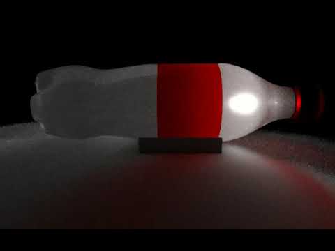
Conventional rendering is referred to as steady state, where the light propagation speed is assumed to be infinite. In contrast, transient rendering breaks this assumption allowing us to simulate light in motion (see the teaser image for a visual example).

For example, path tracing algorithms integrate over multiple paths that connect a light source with the camera. For a known path, transient path tracing uses the very complex formula of time = distance / speed (see [Two New Sciences by Galileo]) to compute the time when each photon arrives at the camera from the path's distance and light's speed. This adds a new time dimension to the captured images (i.e. it's a video now). The simulations now take new parameters as input: when to start recording the video, how long is each time step (framerate), and how many frames to record.

Note: note that the time values we need to compute are very small (e.g. light takes only ~3.33 10^-9 seconds to travel 1 meter), time is usually measured in optical path distance. See Wikipedia for more information. TL;DR opl = distance * refractive_index*

Video